💡 New to PPO or GRPO? These introductions are good places to start before reading this blog: PPO and GRPO.

Policy losses, or objectives, in LLM RL usually involve importance ratio. Define the token-level ratio as

where \(\pi_\theta\) is the current policy and \(\pi_{\text{old}}\) is the old policy. The old policy could be the snapshot of the model weights at the beginning of the gradient update, as in PPO, or the rollout policy in asynchronous training such as SAO⁵, lagged by more than one gradient update.

Let’s take PPO for example to see how \(\rho_t\) is used in the RL. The full PPO objective¹ is

To make it simpler, we can consider the token-level objective alone, since the full objective is an expectation of it over trajectories.

The min and clip operations in eq. (3) are where most writeups bury readers in notation. Split the objective by the sign of \(A_t\), then by where \(\rho_t\) sits relative to the clip bounds, and the logic becomes straightforward.

Illustration of PPO

Case \(A_t > 0\)

This token is better than we thought, so we should increase its probability. Indeed,

Unclipped region (\(\rho_t < 1 + \epsilon\))

Increasing the better token probability \(\rho_t\) increases the objective \(J_t\), exactly what we should do for a positive advantage \(A_t\).

Clipped region (\(\rho_t > 1+\epsilon\)).

In other words, it tells us don’t be too greedy if the current policy \(\pi_{\theta}\) already strongly prefers the better token — we should stop assigning more importance to it.

Case \(A_t < 0\)

This token is worse than we thought, so we should decrease its probability. Indeed,

Unclipped region (\(\rho_t \ge 1-\epsilon\))

Decreasing \(\rho_t\) increases \(J_t\), as it should for a negative advantage.

Clipped region (\(\rho_t < 1-\epsilon\)).

Once the policy has already moved far enough against this token, further decreases are clipped out.

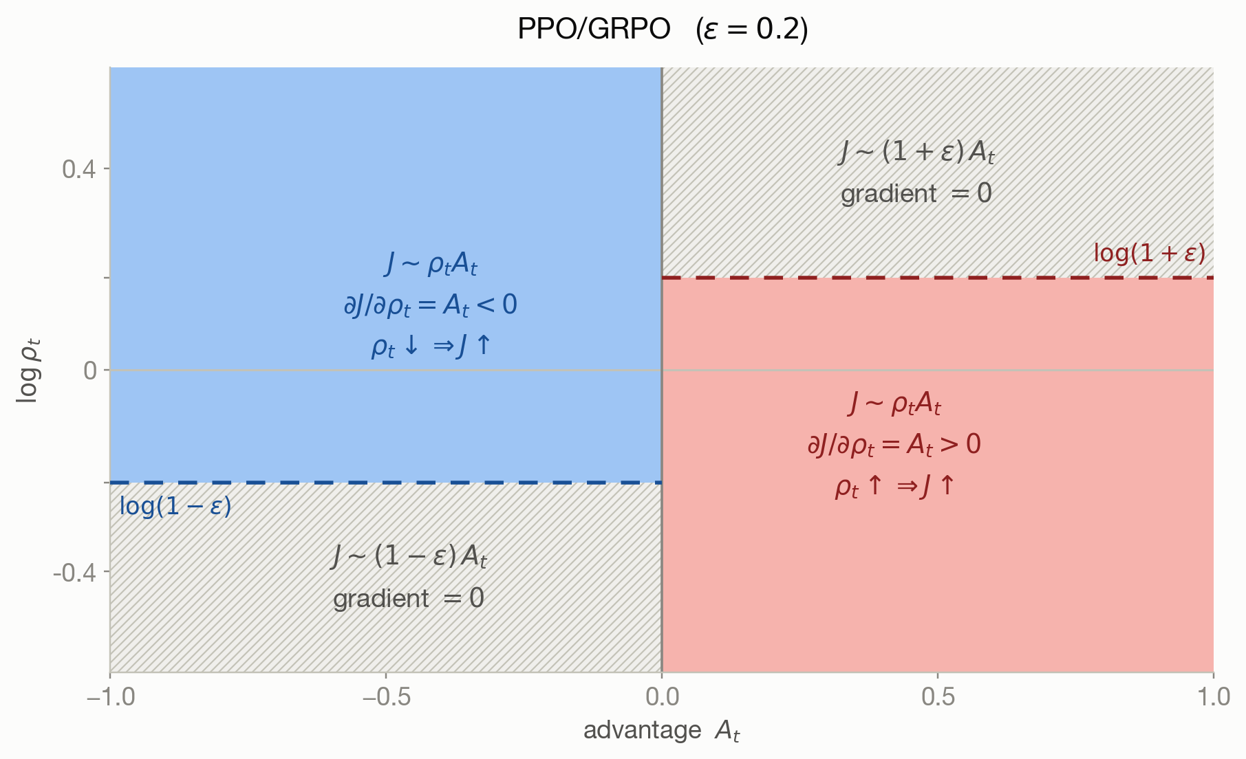
Figure 1 summarizes this behavior. On the \(\log\rho_t\) vs. \(A_t\) plane, a sampled token falls into one of four regions: in the red region, PPO/GRPO encourages the token by increasing its probability; in the blue region, it discourages the token; in the remaining regions, the gradient on \(\rho_t\) is zero, so the token is effectively dropped from the parameter update.

Generalized RL objective

The SAPO paper⁶ gives us a useful way to compare these policy optimization methods. At the token level, write the surrogate objective as

Policy optimization methods, such as PPO/GRPO, DAPO, GSPO, SAO, and SAPO, differ mainly in their choice of the weight function \(f\). Taking the gradient of eq. (4),

All methods share the term \(\rho_t A_t\nabla_\theta\log\pi_\theta\). They only differ in the gate function \(f'(\rho_t;A_t)\) that determines how much learning signal gets through.

Table 1 summarizes the weight function \(f\) and gate function \(f'\) of some milestone policy optimization methods in LLM RL.

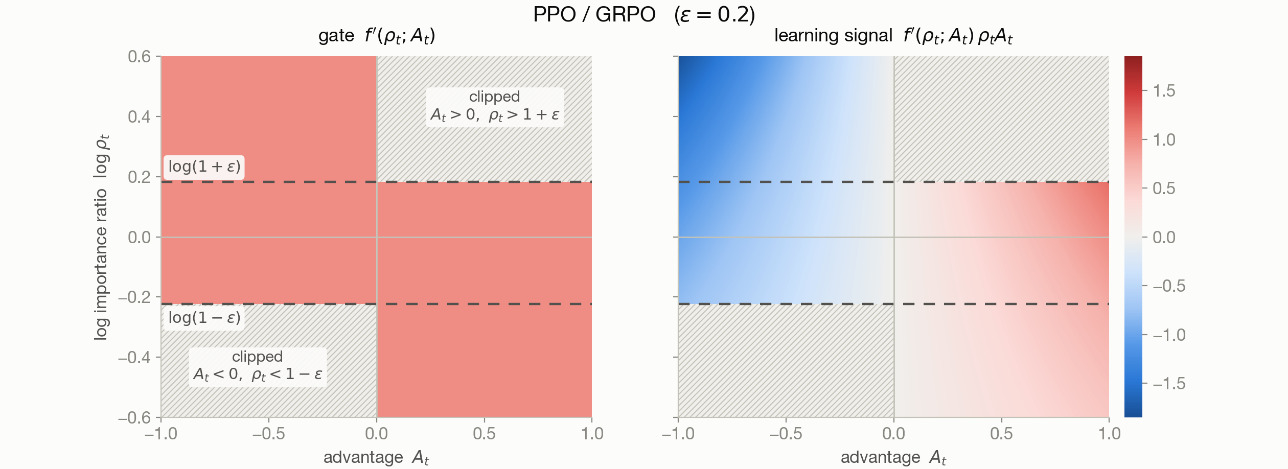
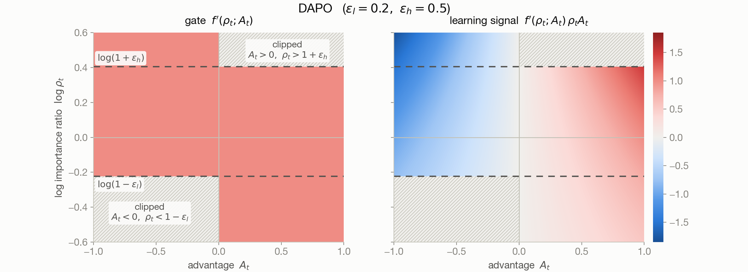
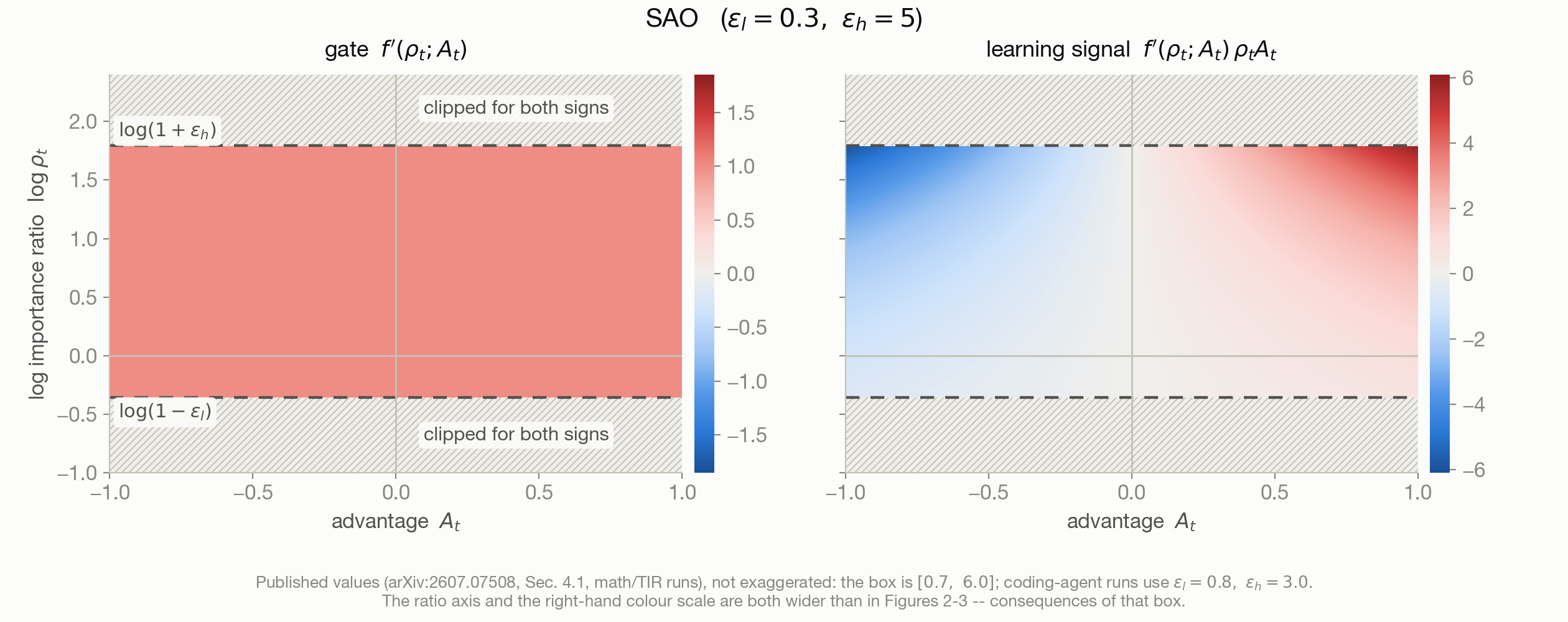
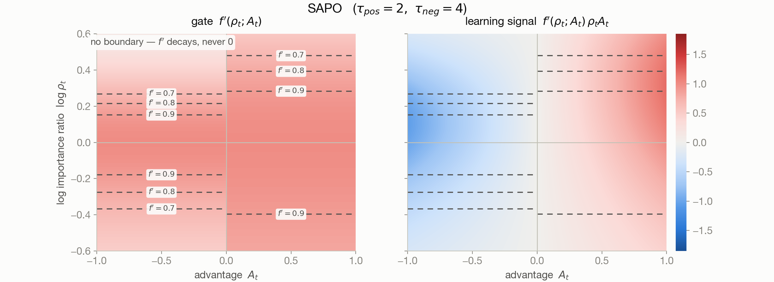
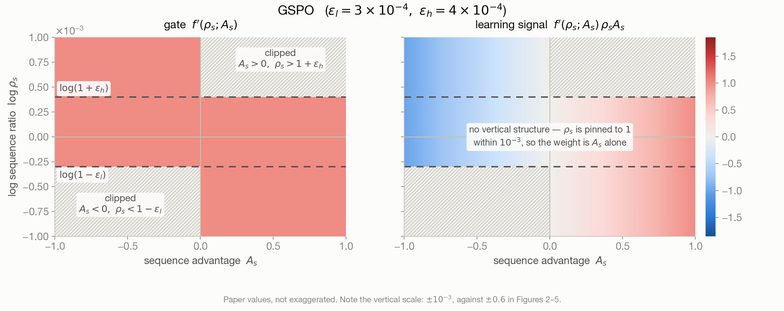
Figures 2–6 plot the gate \(f'(\rho_t;A_t)\) and the learning signal \(f'(\rho_t;A_t)\,\rho_t A_t\) on the \((A_t,\log\rho_t)\) plane for each method (Figure 6 uses the sequence pair \((A_s,\rho_s)\)):

• PPO¹ (Figure 2) clips the importance ratio \(\rho_t\): once an update has encouraged a good token or discouraged a bad token enough, the gate drops to zero and the token stops contributing. This keeps policy updates small and training stable.
• GRPO² (Figure 2) adds a group rollout dimension \(G\) to the objective. At the token level, its gate is identical to PPO’s.
• DAPO³ (Figure 3) raises the upper clipping threshold \(\epsilon_h\), so rare tokens—whose small denominator tends to produce large \(\rho_t\) values—are less likely to be clipped prematurely. The extra strip above PPO’s boundary is exactly where the largest learning signals live.
• SAO⁵ (Figure 4) targets asynchronous training, where the current and rollout policies can drift farther apart than in PPO. \(\rho_t\) can then deviate substantially from 1, so the gate behaves like a top-hat window, masking both signs whenever the ratio leaves the trust region.
• SAPO⁶ (Figure 5) replaces this hard boundary with a smooth gate. Instead of switching off a token’s contribution once \(\rho_t\) crosses a threshold, SAPO lets the weight decay gradually as the ratio moves away from the preferred region.
• GSPO⁴ (Figure 6) is the same move at sequence level: swap \((A_t,\rho_t)\) for sequence level \((A_s,\rho_s)\) with \(\rho_s=(\pi_\theta(y\mid x)/\pi_{\mathrm{old}}(y\mid x))^{1/\lvert y\rvert}\)—the geometric mean of the token ratios in eq. (1). Note that the shared factor changes as well: \(\nabla_\theta\rho_s=\rho_s\cdot\frac{1}{\lvert y\rvert}\sum_t\nabla_\theta\log\pi_\theta(y_t\mid x,y_{<t})\), i.e. every token in the response receives the same length-averaged weight. The gate is DAPO’s asymmetric two-wedge shape, but with GSPO’s clip range (\(\epsilon\sim 3\text{–}4\times10^{-4}\)) \(\rho_s\) stays within \(10^{-3}\) of 1, so the learning signal is essentially \(A_s\) alone.

Takeaways

Using SAPO’s⁶ generalized form of objective \(J\) with weight function \(f(\rho_t; A_t)\), learning signals of different RL methods can be shown on the same \((A_t,\log\rho_t)\) plane.

• PPO / GRPO: hard token-level gate.
• DAPO: widens the gate for useful low-probability tokens.
• SAO: keeps only ratios inside a trust region when rollout policies become stale.
• SAPO: turns the hard gate into a smooth one.
• GSPO: moves the same idea from tokens to sequences.

Seen this way, these methods are providing different answers to the same question: which policy-gradient signals should we trust, and how much?

where \(Z(x)\) is the partition function defined in eq. (13). This same structure underlies DPO’s derivation¹ and KL-regularized RLHF methods such as PPO- and GRPO-style training.²

Most explanations—including Karina Zadorozhny’s post-training guide and Ari G’s RLHF-to-DPO walkthrough—essentially stop there. They introduce \(Z(x)\), note its connection to statistical physics, observe that it is intractable but conveniently cancels from the pairwise DPO loss, derive the optimal policy in eq. (1), and move on.

But in statistical mechanics, writing down the partition function is not the end of the derivation. It is the beginning. Once \(Z\) is defined in eq. (13), free energy, internal energy, entropy, and temperature follow, together with a precise characterization of equilibrium. The KL-regularized RL objective admits an almost term-by-term version of the same structure.

This post works out that dictionary explicitly: reward as negative energy, \(\beta\) as temperature, KL divergence as relative entropy, and the RL objective as a free-energy principle in eq. (4). Then I ask the question the analogy naturally suggests: if the theory predicts a unique Gibbs optimum \(\pi_\beta^\ast\) in eq. (1), how close does actual training get to it? I test this with a GRPO-family trainer³ on GSM8K.

The KL-regularized objective

Equation (3) in Rafailov et al. (2023)¹ defines the KL-regularized RLHF objective that underlies DPO. The same reward–KL tradeoff appears in PPO and GRPO; those methods optimize surrogates or sample-based estimators plus a KL divergence term for regularization with respect to reference policy. In general, for a fixed prompt \(x\), the goal is to optimize

For readability, we suppress the conditioning on \(x\) and write \(\pi(y)\equiv\pi(y\mid x)\), \(\pi_{\mathrm{ref}}(y)\equiv\pi_{\mathrm{ref}}(y\mid x)\), and \(r(y)\equiv r(x,y)\). The objective becomes

Maximizing \(J[\pi]\) is equivalent to minimizing

Here \(\mathcal{F}_{\beta}\) is a functional of the policy \(\pi\). Given a reference policy \(\pi_{\mathrm{ref}}\) and reward function \(r\), the problem is to find the policy \(\pi\) that minimizes eq. (4).

Mapping to statistical mechanics

The objective in eq. (4) has the form of a Helmholtz free energy. Each response \(y\) is a state of the system, with energy

For a policy \(\pi\), define the mean energy and dimensionless relative entropy as

This objective is therefore

which matches \(F=U-TS\) term by term:

Here DPO’s \(\beta\) plays the role of thermal energy \(k_B T\), so its Boltzmann factor \(e^{-\epsilon/\beta}\) matches \(e^{-\beta_{\mathrm{phys}}\epsilon}\) under the physics convention \(\beta_{\mathrm{phys}}=1/(k_B T)\).

But shouldn’t entropy be \(-\sum_{i}\pi_i\log{\pi_i}\)? Why does it involve a reference distribution, \(-\sum_{i}\pi_i\log{\pi_i/\pi_{\mathrm{ref},i}}\)? Ordinary entropy takes exactly this form when states have degeneracies. Suppose coarse-grained state \(i\) contains \(g_i\) microstates and has total probability \(\pi_i\). If those microstates are equally likely, each has probability \(p_{i,\alpha}=\pi_i/g_i\), so

Let \(G=\sum_j g_j\) and normalize the degeneracies as \(q_i=g_i/G\). Expanding the logarithm,

The constant \(\log G\) does not affect minimization of the free energy in eq. (4). Thus, up to an additive constant, degeneracy turns ordinary entropy into negative KL divergence relative to the normalized degeneracy measure \(q\).

Minimizing \(F=U-TS/k_B=\sum_i\pi_i\epsilon_i+\beta D_{\mathrm{KL}}(\pi\|q)\) subject to \(\sum_i\pi_i=1\) (the same variational problem as in Appendix B, with \(\pi_{\mathrm{ref}}\) replaced by \(q\)) gives the Boltzmann distribution

This is the standard form for degenerate systems; see Ellgen, Thermodynamics and Chemical Equilibrium, §21.1 and Pathria and Beale, Statistical Mechanics, §3.4.

In KL-regularized RL, \(\pi_{\mathrm{ref}}(y)\) is the normalized degeneracy measure \(q(y)\). With \(\epsilon(y)=-r(y)\) from eq. (5) and DPO’s \(\beta\) corresponding to thermal energy \(k_B T\) (so \(\beta_{\mathrm{phys}}=1/\beta\)),

which is the Boltzmann weight appearing in eq. (1).

The Gibbs optimum

In statistical mechanics, for fixed temperature, energy levels, and normalized degeneracy measure \(q\), the Gibbs distribution uniquely minimizes the free energy. The same variational principle holds here: once \(\beta\), the reward function, and the reference policy \(\pi_{\mathrm{ref}}\) are fixed, there is a unique optimal policy that minimizes \(\mathcal{F}_{\beta}\) in eq. (4). In a physical system, \(q\) is fixed by degeneracies; in preference optimization, \(\pi_{\mathrm{ref}}\) is a modeling choice that may vary across setups, but within any one setup it serves as the fixed reference.

Following the steps in the appendix, the free energy decomposes as

where the partition function is

and the corresponding Gibbs policy is eq. (1), with \(Z(x)\) replaced by \(Z_{\beta}\) when conditioning on \(x\) is suppressed.

Since \(D_{\mathrm{KL}}(\pi\|\pi_{\beta}^{\ast})\ge 0\), with equality if and only if \(\pi=\pi_{\beta}^{\ast}\), the unique minimizer is \(\pi_{\beta}^{\ast}\) and the equilibrium free energy is \(\mathcal{F}_{\beta}^{\ast}=-\beta\log Z_{\beta}\). This is exactly the free energy of a canonical ensemble. More generally, once the partition function in eq. (13) is known, equilibrium quantities such as internal energy, entropy, and heat capacity follow from it and its derivatives with respect to \(\beta\)—the same logic summarized in the dictionary below and in eq. (8).

There are two standard ways to derive \(\pi_{\beta}^{\ast}\):

1. Partition-function / KL decomposition. Rewrite eq. (4) so that an unnormalized Boltzmann weight appears, then normalize it by \(Z_{\beta}\) from eq. (13).
2. Lagrange multiplier. Enforce the normalization constraint \(\sum_y\pi(y)=1\) while setting the functional derivative of \(\mathcal{F}_{\beta}\) to zero; the stationary point is again eq. (1).

Full algebra for both routes is in the appendix.

The dictionary

Statistical mechanics on the left, KL-regularized RL on the right:

The heat-capacity entry follows from differentiating the partition function in eq. (13). Write \(t=1/\beta\) so that \(Z_{\beta}=\sum_y\pi_{\mathrm{ref}}(y)e^{tr(y)}\). Standard identities for the Gibbs policy in eq. (1) give \(\mathbb{E}_{\pi_{\beta}^{\ast}}[r]=\partial_t\log Z_{\beta}\) and \(\operatorname{Var}_{\pi_{\beta}^{\ast}}[r]=\partial_t^2\log Z_{\beta}\). Since \(t=1/\beta\) implies \(\mathrm{d}t/\mathrm{d}\beta=-1/\beta^2\),

With \(\epsilon=-r\), this is the usual canonical-ensemble relation \(C_V/k_B=\beta_{\mathrm{phys}}^2\operatorname{Var}(\epsilon)\).

Experiments on GSM8K

Everything above is exact at the level of probability distributions. To see what that ideal predicts for a real model, I ran Qwen2.5-0.5B-Instruct on GSM8K with a binary reward: \(r(y)=1\) when the final answer is correct and \(0\) otherwise.

The Gibbs floor

For each of 64 GSM8K test prompts \(x_i\), I sampled 24 candidate responses \(y_{ij}\) from the base model, giving 1,536 completions in total. Generation used temperature 0.8, top-p 0.95, and a 512-token limit. Each candidate has a base-model log-probability and a binary correctness reward \(r(x_i,y_{ij})\in\{0,1\}\). Normalizing the base-model probabilities over the 24 candidates defines \(\pi_{\mathrm{ref}}(y_{ij}\mid x_i)\) on this finite candidate set.

Treating these 24 candidates as the state space turns every expectation into a finite sum. For each prompt, eqs. (1) and (13) become

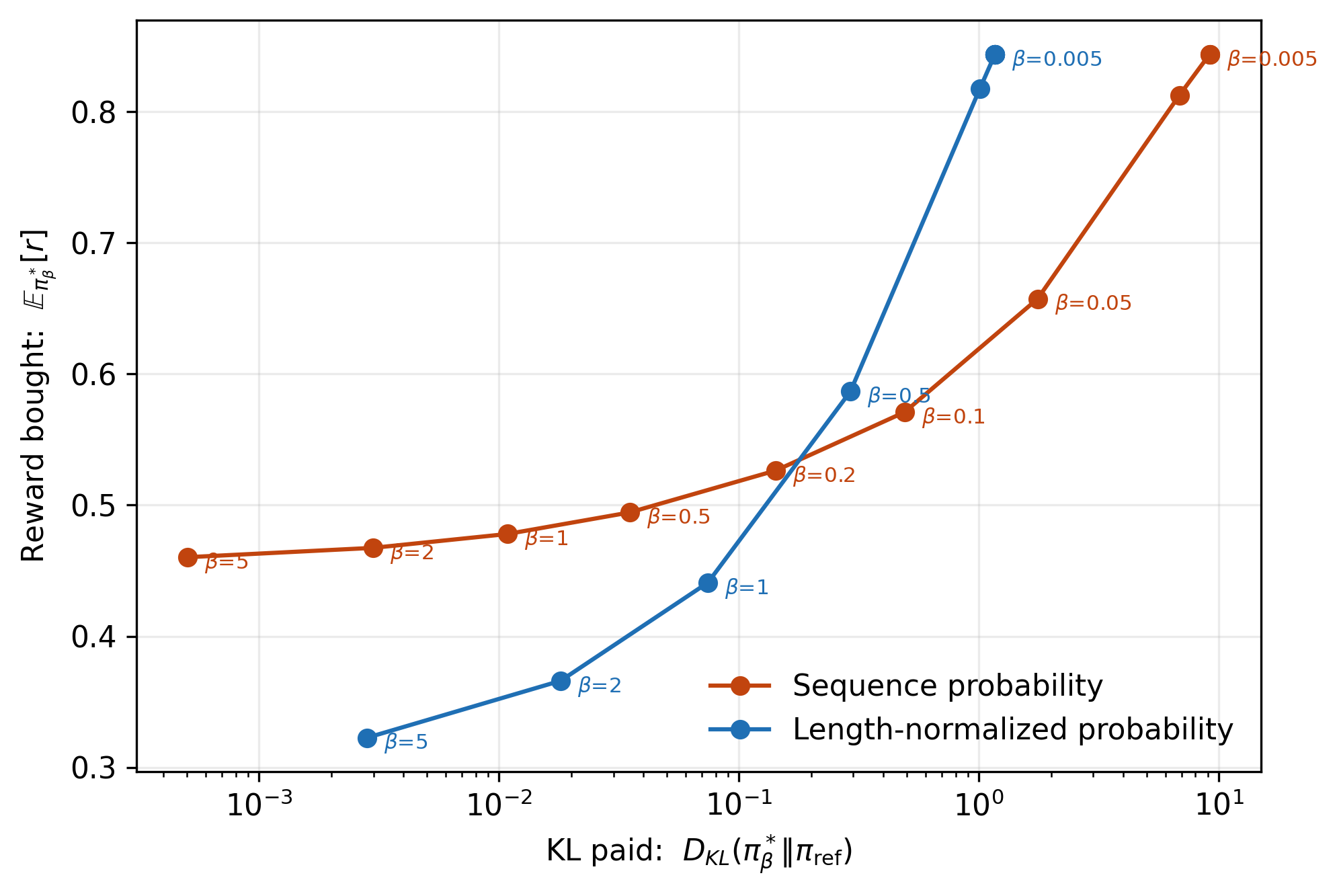
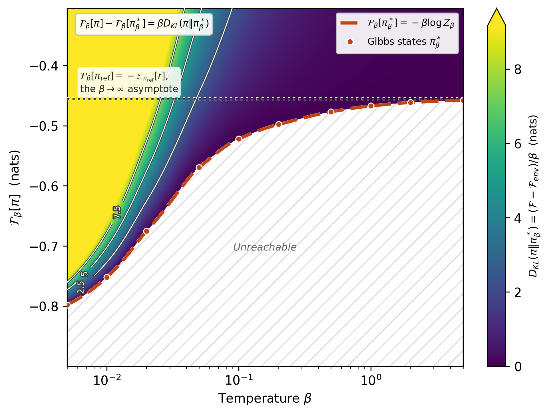
Once the candidate set has been sampled, the Gibbs policy and its expected reward, KL divergence, and free energy from eq. (4) can all be evaluated exactly on that set. Sweeping \(\beta\) traces the optimal reward–KL frontier in Figure 1 and the corresponding free-energy landscape in Figure 2. Figure 1 also compares two ways of defining the reference weights: full-sequence probability and length-normalized probability. The remaining experiments use full-sequence probability.

GRPO-family training vs. the floor

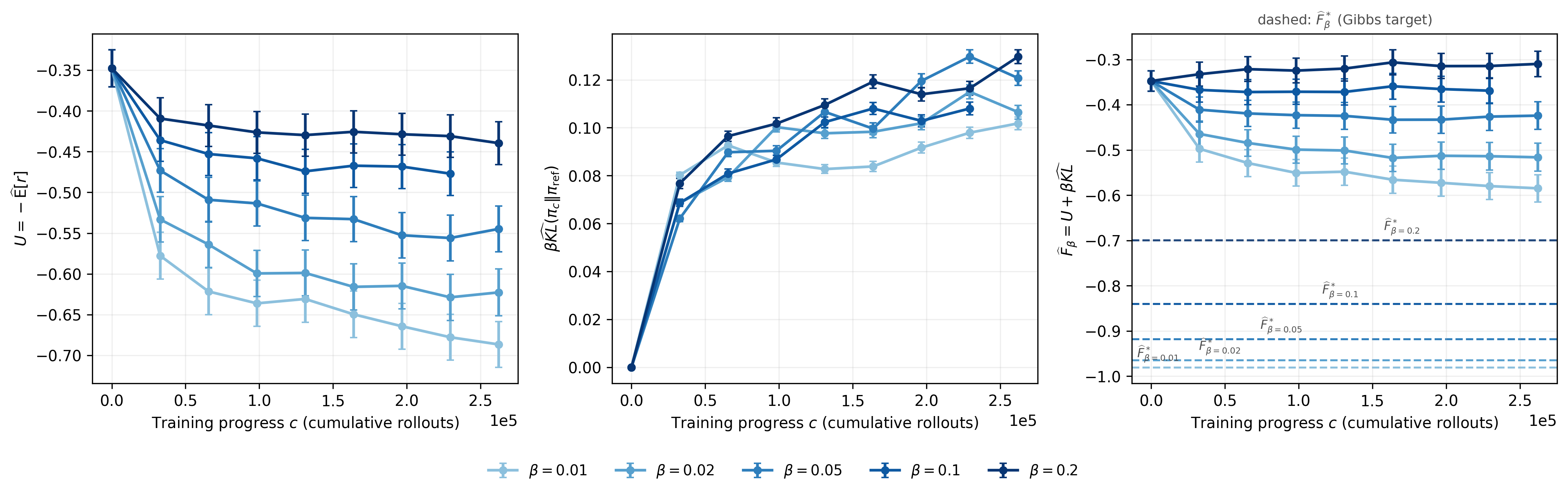
At the reference policy the KL term is zero, so \(\mathcal{F}_{\beta}[\pi_{\mathrm{ref}}]=-\mathbb{E}_{\pi_{\mathrm{ref}}}[r]\), shown as the black dotted baseline in Figure 2. If training reaches the distribution-level optimum, its free energy should fall from this baseline toward the red Gibbs minimum at \(\mathcal{F}_{\beta}^{\ast}=-\beta\log Z_{\beta}\) from eq. (12).

To test this, I ran a GRPO-family trainer³ separately for \(\beta\in\{0.01,0.02,0.05,0.1,0.2\}\), using group size \(G=32\), 6,500 GSM8K training prompts, for about one epoch (262,144 rollouts). I saved checkpoints every 32,768 rollouts and evaluated each checkpoint on the same 500 held-out prompts. The reference model starts at an expected reward of 0.348.

Why training falls short

I expected each policy to move toward its \(\pi_{\beta}^{\ast}\) from eq. (1) and each free-energy curve to approach its dashed target from eq. (12). Figure 3 shows that this was too optimistic: after one epoch, none of the runs reached its Gibbs minimum. Reward improved, but not enough to offset the accompanying \(\beta\)-weighted KL cost, so the measured free energy stayed above the target.

Likely explanations:

1. Limited expressivity. Optimization is restricted to the parameter space of a 0.5B model, which may not contain the true Gibbs policy.
2. Non-convex loss. Even within that parameter space, the loss is non-convex, so gradient descent is not guaranteed to find the global minimum.

Takeaways

• KL-regularized RL is free-energy minimization in statistical physics: eq. (4) is the RL free energy and eq. (8) is the dictionary.
  • Given \(\beta\), reference policy \(\pi_{\mathrm{ref}}\), and reward function \(r\), there is a unique policy \(\pi_{\beta}^{\ast}\) in eq. (1) that minimizes the free energy.
  • From \(Z_{\beta}\) in eq. (13) we can read off internal energy, entropy, temperature, free energy, and heat capacity.
• Training may not reach that distribution-level optimum.

Code and full experiments: github.com/wang-zhongwei/stat-mech-dpo

Appendix: two derivations of the optimal policy

Both routes start from eq. (4), equivalently written as

and the normalization constraint \(\sum_y\pi(y)=1\). They recover the partition function in eq. (13), the optimal policy in eq. (1), and the free-energy minimum in eq. (12).

A. Partition-function / KL decomposition

Writing the expectation and KL divergence explicitly and dividing by \(\beta\) gives

The Boltzmann weight \(\pi_{\mathrm{ref}}(y)e^{r(y)/\beta}\) from eq. (11) appears directly from the objective—not as an ansatz. Normalizing it by the partition function in eq. (13) gives the optimal policy in eq. (1).

Substituting \(\pi_{\mathrm{ref}}(y)e^{r(y)/\beta}=Z_{\beta}\pi_{\beta}^{\ast}(y)\) then yields

Because \(\pi\) is a normalized probability distribution, \(\sum_y\pi(y)=1\). Multiplying by \(\beta\) therefore gives eq. (12):

Since \(D_{\mathrm{KL}}(\pi\|\pi_{\beta}^{\ast})\ge 0\), with equality if and only if \(\pi=\pi_{\beta}^{\ast}\), the unique minimizer is eq. (1) and \(\mathcal{F}_{\beta}^{\ast}=-\beta\log Z_{\beta}\).

With \(\epsilon=-r\) from eq. (5), the same algebra produces the statistical-mechanics form

For a uniform \(\pi_{\mathrm{ref}}\), this reduces to the canonical Gibbs distribution \(e^{-\epsilon/\beta}/Z_{\beta}\).

B. Lagrange multiplier

To minimize eq. (4) subject to \(\sum_y\pi(y)=1\), introduce a Lagrange multiplier \(\lambda\):

Stationarity with respect to each \(\pi(y)\) requires

Solving for \(\pi(y)\) gives

where \(C=e^{-1-\lambda/\beta}\) is independent of \(y\). Enforcing normalization yields \(C^{-1}=Z_{\beta}\) from eq. (13), and therefore the same optimal policy as eq. (1):

Substituting this stationary point back into eq. (4) recovers the equilibrium free energy \(\mathcal{F}_{\beta}^{\ast}=-\beta\log Z_{\beta}\) from eq. (12).