A Statistical Mechanics View of KL-Regularized RL

Preference post-training is often formulated as KL-regularized reward maximization: increase expected reward while staying close to a reference policy. Its optimum takes the Gibbs form

$$\pi_\beta^\ast(y|x) = \frac{\pi_{\mathrm{ref}}(y|x)e^{r(x,y)/\beta}}{Z(x)}, \tag{1}$$

where $Z(x)$ is the partition function defined in eq. (13). This same structure underlies DPO’s derivation¹ and KL-regularized RLHF methods such as PPO- and GRPO-style training.²

Most explanations—including Karina Zadorozhny’s post-training guide and Ari G’s RLHF-to-DPO walkthrough—essentially stop there. They introduce $Z(x)$, note its connection to statistical physics, observe that it is intractable but conveniently cancels from the pairwise DPO loss, derive the optimal policy in eq. (1), and move on.

But in statistical mechanics, writing down the partition function is not the end of the derivation. It is the beginning. Once $Z$ is defined in eq. (13), free energy, internal energy, entropy, and temperature follow, together with a precise characterization of equilibrium. The KL-regularized RL objective admits an almost term-by-term version of the same structure.

This post works out that dictionary explicitly: reward as negative energy, $\beta$ as temperature, KL divergence as relative entropy, and the RL objective as a free-energy principle in eq. (4). Then I ask the question the analogy naturally suggests: if the theory predicts a unique Gibbs optimum $\pi_\beta^\ast$ in eq. (1), how close does actual training get to it? I test this with a GRPO-family trainer³ on GSM8K.

The KL-regularized objective

Equation (3) in Rafailov et al. (2023)¹ defines the KL-regularized RLHF objective that underlies DPO. The same reward–KL tradeoff appears in PPO and GRPO; those methods optimize surrogates or sample-based estimators plus a KL divergence term for regularization with respect to reference policy. In general, for a fixed prompt $x$, the goal is to optimize

$$\max_{\pi} \; \mathbb{E}_{y\sim\pi(\cdot\mid x)} \left[ r(x,y) \right] - \beta D_{\mathrm{KL}} \left( \pi(\cdot\mid x) \;\|\; \pi_{\mathrm{ref}}(\cdot\mid x) \right). \tag{2}$$

For readability, we suppress the conditioning on $x$ and write $\pi(y)\equiv\pi(y\mid x)$, $\pi_{\mathrm{ref}}(y)\equiv\pi_{\mathrm{ref}}(y\mid x)$, and $r(y)\equiv r(x,y)$. The objective becomes

$$J[\pi] = \mathbb{E}_{y\sim\pi}[r(y)] - \beta D_{\mathrm{KL}} \left( \pi \;\|\; \pi_{\mathrm{ref}} \right). \tag{3}$$

Maximizing $J[\pi]$ is equivalent to minimizing

$$\boxed{ \mathcal{F}_{\beta}[\pi] = - \mathbb{E}_{y\sim\pi}[r(y)] + \beta D_{\mathrm{KL}} \left( \pi \;\|\; \pi_{\mathrm{ref}} \right). } \tag{4}$$

Here $\mathcal{F}_{\beta}$ is a functional of the policy $\pi$. Given a reference policy $\pi_{\mathrm{ref}}$ and reward function $r$, the problem is to find the policy $\pi$ that minimizes eq. (4).

Mapping to statistical mechanics

The objective in eq. (4) has the form of a Helmholtz free energy. Each response $y$ is a state of the system, with energy

$$\epsilon(y)=-r(y). \tag{5}$$

For a policy $\pi$, define the mean energy and dimensionless relative entropy as

$$U[\pi]=\mathbb{E}_{\pi}[\epsilon]=-\mathbb{E}_{\pi}[r], \qquad S_{\mathrm{rel}}[\pi]=-D_{\mathrm{KL}}(\pi\|\pi_{\mathrm{ref}}). \tag{6}$$

This objective is therefore

$$\mathcal{F}_{\beta}[\pi] =U[\pi]-\beta S_{\mathrm{rel}}[\pi], \tag{7}$$

which matches $F=U-TS$ term by term:

$$\boxed{ \epsilon(y)\longleftrightarrow-r(y),\qquad k_B T\longleftrightarrow\beta,\qquad \frac{S}{k_B}\longleftrightarrow-D_{\mathrm{KL}}(\pi\|\pi_{\mathrm{ref}}). } \tag{8}$$

Here DPO’s $\beta$ plays the role of thermal energy $k_B T$, so its Boltzmann factor $e^{-\epsilon/\beta}$ matches $e^{-\beta_{\mathrm{phys}}\epsilon}$ under the physics convention $\beta_{\mathrm{phys}}=1/(k_B T)$.

But shouldn’t entropy be $-\sum_{i}\pi_i\log{\pi_i}$? Why does it involve a reference distribution, $-\sum_{i}\pi_i\log{\pi_i/\pi_{\mathrm{ref},i}}$? Ordinary entropy takes exactly this form when states have degeneracies. Suppose coarse-grained state $i$ contains $g_i$ microstates and has total probability $\pi_i$. If those microstates are equally likely, each has probability $p_{i,\alpha}=\pi_i/g_i$, so

$$\frac{S}{k_B} =-\sum_{i,\alpha}p_{i,\alpha}\log p_{i,\alpha} =-\sum_i\pi_i\log\frac{\pi_i}{g_i}.$$

Let $G=\sum_j g_j$ and normalize the degeneracies as $q_i=g_i/G$. Expanding the logarithm,

$$\frac{S}{k_B} = -\sum_i \pi_i \log\pi_i + \sum_i \pi_i \log g_i = -\sum_i \pi_i \log\frac{\pi_i}{q_i} + \log G = -D_{\mathrm{KL}}(\pi\|q)+\log G. \tag{9}$$

The constant $\log G$ does not affect minimization of the free energy in eq. (4). Thus, up to an additive constant, degeneracy turns ordinary entropy into negative KL divergence relative to the normalized degeneracy measure $q$.

Minimizing $F=U-TS/k_B=\sum_i\pi_i\epsilon_i+\beta D_{\mathrm{KL}}(\pi\|q)$ subject to $\sum_i\pi_i=1$ (the same variational problem as in Appendix B, with $\pi_{\mathrm{ref}}$ replaced by $q$) gives the Boltzmann distribution

$$\pi_i = \frac{g_i \exp(-\beta_{\mathrm{phys}} \epsilon_i)}{Z}, \qquad Z = \sum_{i} g_i \exp(-\beta_{\mathrm{phys}} \epsilon_i). \tag{10}$$

This is the standard form for degenerate systems; see Ellgen, Thermodynamics and Chemical Equilibrium, §21.1 and Pathria and Beale, Statistical Mechanics, §3.4.

In KL-regularized RL, $\pi_{\mathrm{ref}}(y)$ is the normalized degeneracy measure $q(y)$. With $\epsilon(y)=-r(y)$ from eq. (5) and DPO’s $\beta$ corresponding to thermal energy $k_B T$ (so $\beta_{\mathrm{phys}}=1/\beta$),

$$e^{-\beta_{\mathrm{phys}}\epsilon}=e^{r/\beta}, \tag{11}$$

which is the Boltzmann weight appearing in eq. (1).

The Gibbs optimum

In statistical mechanics, for fixed temperature, energy levels, and normalized degeneracy measure $q$, the Gibbs distribution uniquely minimizes the free energy. The same variational principle holds here: once $\beta$, the reward function, and the reference policy $\pi_{\mathrm{ref}}$ are fixed, there is a unique optimal policy that minimizes $\mathcal{F}_{\beta}$ in eq. (4). In a physical system, $q$ is fixed by degeneracies; in preference optimization, $\pi_{\mathrm{ref}}$ is a modeling choice that may vary across setups, but within any one setup it serves as the fixed reference.

Following the steps in the appendix, the free energy decomposes as

$$\boxed{ \mathcal{F}_{\beta}[\pi] = -\beta\log Z_{\beta} + \beta D_{\mathrm{KL}} \left( \pi \;\|\; \pi_{\beta}^{\ast} \right). } \tag{12}$$

where the partition function is

$$\boxed{ Z_{\beta} = \sum_y \pi_{\mathrm{ref}}(y) e^{r(y)/\beta} } \tag{13}$$

and the corresponding Gibbs policy is eq. (1), with $Z(x)$ replaced by $Z_{\beta}$ when conditioning on $x$ is suppressed.

Since $D_{\mathrm{KL}}(\pi\|\pi_{\beta}^{\ast})\ge 0$, with equality if and only if $\pi=\pi_{\beta}^{\ast}$, the unique minimizer is $\pi_{\beta}^{\ast}$ and the equilibrium free energy is $\mathcal{F}_{\beta}^{\ast}=-\beta\log Z_{\beta}$. This is exactly the free energy of a canonical ensemble. More generally, once the partition function in eq. (13) is known, equilibrium quantities such as internal energy, entropy, and heat capacity follow from it and its derivatives with respect to $\beta$—the same logic summarized in the dictionary below and in eq. (8).

There are two standard ways to derive $\pi_{\beta}^{\ast}$:

1. Partition-function / KL decomposition. Rewrite eq. (4) so that an unnormalized Boltzmann weight appears, then normalize it by $Z_{\beta}$ from eq. (13).
2. Lagrange multiplier. Enforce the normalization constraint $\sum_y\pi(y)=1$ while setting the functional derivative of $\mathcal{F}_{\beta}$ to zero; the stationary point is again eq. (1).

Full algebra for both routes is in the appendix.

The dictionary

Statistical mechanics on the left, KL-regularized RL on the right:

Statistical mechanics	KL-regularized RL
Energy of state $\epsilon$	$-r$ (negative reward)
Normalized degeneracy $q$	$\pi_{\mathrm{ref}}$
Internal energy $U$	$-\mathbb{E}_{\pi}[r]$
Entropy $S$	$-D_{\mathrm{KL}}(\pi \Vert \pi_{\mathrm{ref}})$
Temperature $k_B T$	DPO’s $\beta$
Partition function $Z$	$\sum_y \pi_{\mathrm{ref}}(y)\,e^{r(y)/\beta}$
Minimum free energy $F^{\ast}$	$-\beta \log Z_\beta$
Free-energy gap	$\beta\, D_{\mathrm{KL}}(\pi \Vert \pi_\beta^{\ast})$
Heat capacity $C_V/k_B$	$\displaystyle \frac{\operatorname{Var}_{\pi_{\beta}^{\ast}}[r]}{\beta^2} = -\frac{\partial \mathbb{E}_{\pi_{\beta}^{\ast}}[r]}{\partial \beta}$

The heat-capacity entry follows from differentiating the partition function in eq. (13). Write $t=1/\beta$ so that $Z_{\beta}=\sum_y\pi_{\mathrm{ref}}(y)e^{tr(y)}$. Standard identities for the Gibbs policy in eq. (1) give $\mathbb{E}_{\pi_{\beta}^{\ast}}[r]=\partial_t\log Z_{\beta}$ and $\operatorname{Var}_{\pi_{\beta}^{\ast}}[r]=\partial_t^2\log Z_{\beta}$. Since $t=1/\beta$ implies $\mathrm{d}t/\mathrm{d}\beta=-1/\beta^2$,

$$-\frac{\partial \mathbb{E}_{\pi_{\beta}^{\ast}}[r]}{\partial \beta} = -\frac{\mathrm{d}t}{\mathrm{d}\beta}\,\frac{\partial \mathbb{E}_{\pi_{\beta}^{\ast}}[r]}{\partial t} = \frac{\operatorname{Var}_{\pi_{\beta}^{\ast}}[r]}{\beta^2}.$$

With $\epsilon=-r$, this is the usual canonical-ensemble relation $C_V/k_B=\beta_{\mathrm{phys}}^2\operatorname{Var}(\epsilon)$.

Experiments on GSM8K

Everything above is exact at the level of probability distributions. To see what that ideal predicts for a real model, I ran Qwen2.5-0.5B-Instruct on GSM8K with a binary reward: $r(y)=1$ when the final answer is correct and $0$ otherwise.

The Gibbs floor

For each of 64 GSM8K test prompts $x_i$, I sampled 24 candidate responses $y_{ij}$ from the base model, giving 1,536 completions in total. Generation used temperature 0.8, top-p 0.95, and a 512-token limit. Each candidate has a base-model log-probability and a binary correctness reward $r(x_i,y_{ij})\in\{0,1\}$. Normalizing the base-model probabilities over the 24 candidates defines $\pi_{\mathrm{ref}}(y_{ij}\mid x_i)$ on this finite candidate set.

Treating these 24 candidates as the state space turns every expectation into a finite sum. For each prompt, eqs. (1) and (13) become

$$Z_{\beta}(x_i) =\sum_{j=1}^{24}\pi_{\mathrm{ref}}(y_{ij}\mid x_i) e^{r(x_i,y_{ij})/\beta}, \qquad \pi_{\beta}^{\ast}(y_{ij}\mid x_i) =\frac{\pi_{\mathrm{ref}}(y_{ij}\mid x_i)e^{r(x_i,y_{ij})/\beta}} {Z_{\beta}(x_i)}. \tag{14}$$

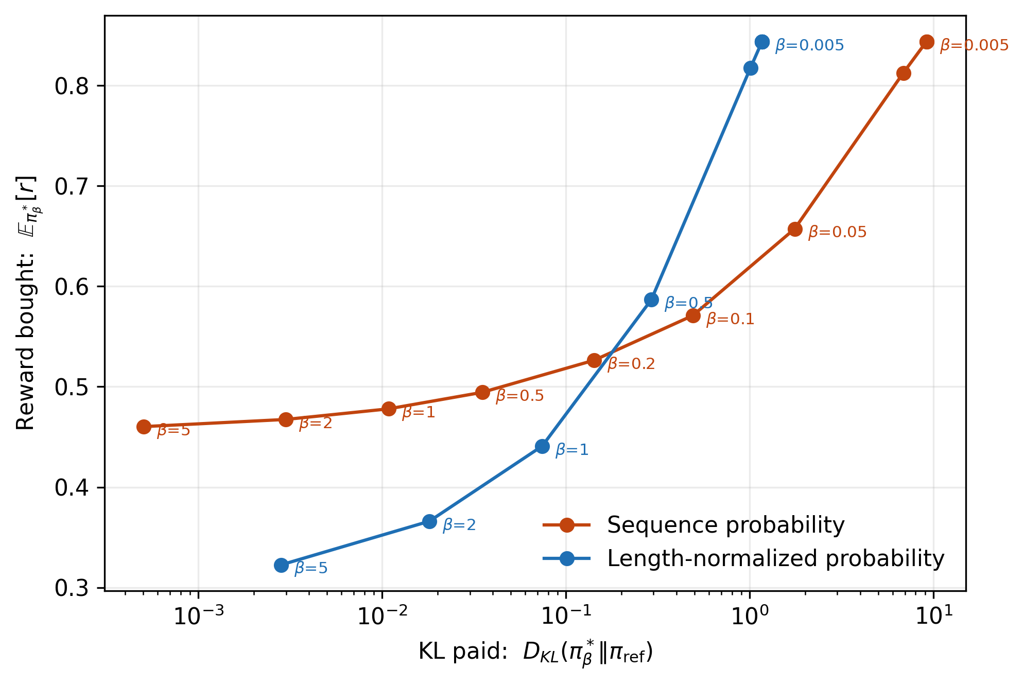
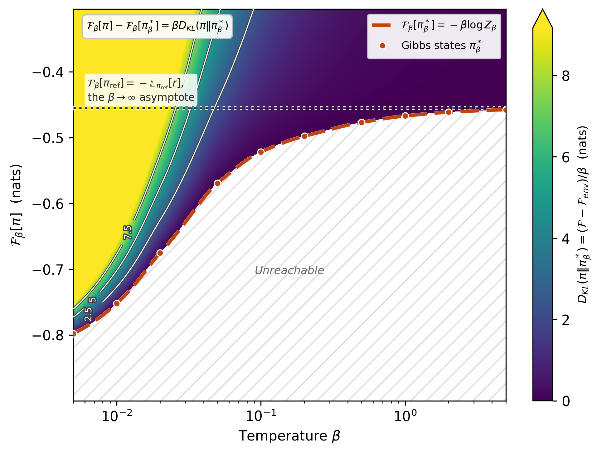
Once the candidate set has been sampled, the Gibbs policy and its expected reward, KL divergence, and free energy from eq. (4) can all be evaluated exactly on that set. Sweeping $\beta$ traces the optimal reward–KL frontier in Figure 1 and the corresponding free-energy landscape in Figure 2. Figure 1 also compares two ways of defining the reference weights: full-sequence probability and length-normalized probability. The remaining experiments use full-sequence probability.

GRPO-family training vs. the floor

At the reference policy the KL term is zero, so $\mathcal{F}_{\beta}[\pi_{\mathrm{ref}}]=-\mathbb{E}_{\pi_{\mathrm{ref}}}[r]$, shown as the black dotted baseline in Figure 2. If training reaches the distribution-level optimum, its free energy should fall from this baseline toward the red Gibbs minimum at $\mathcal{F}_{\beta}^{\ast}=-\beta\log Z_{\beta}$ from eq. (12).

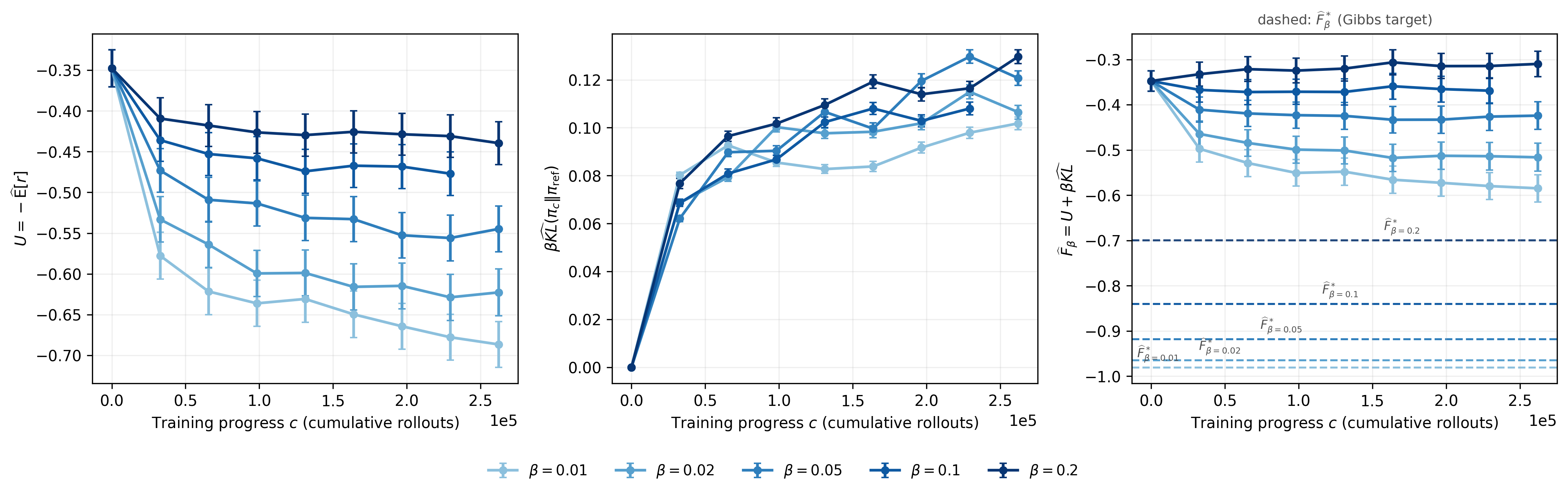
To test this, I ran a GRPO-family trainer³ separately for $\beta\in\{0.01,0.02,0.05,0.1,0.2\}$, using group size $G=32$, 6,500 GSM8K training prompts, for about one epoch (262,144 rollouts). I saved checkpoints every 32,768 rollouts and evaluated each checkpoint on the same 500 held-out prompts. The reference model starts at an expected reward of 0.348.

Why training falls short

I expected each policy to move toward its $\pi_{\beta}^{\ast}$ from eq. (1) and each free-energy curve to approach its dashed target from eq. (12). Figure 3 shows that this was too optimistic: after one epoch, none of the runs reached its Gibbs minimum. Reward improved, but not enough to offset the accompanying $\beta$-weighted KL cost, so the measured free energy stayed above the target.

Likely explanations:

1. Limited expressivity. Optimization is restricted to the parameter space of a 0.5B model, which may not contain the true Gibbs policy.
2. Non-convex loss. Even within that parameter space, the loss is non-convex, so gradient descent is not guaranteed to find the global minimum.

Takeaways

• KL-regularized RL is free-energy minimization in statistical physics: eq. (4) is the RL free energy and eq. (8) is the dictionary.
  • Given $\beta$, reference policy $\pi_{\mathrm{ref}}$, and reward function $r$, there is a unique policy $\pi_{\beta}^{\ast}$ in eq. (1) that minimizes the free energy.
  • From $Z_{\beta}$ in eq. (13) we can read off internal energy, entropy, temperature, free energy, and heat capacity.
• Training may not reach that distribution-level optimum.

Code and full experiments: github.com/wang-zhongwei/stat-mech-dpo

Appendix: two derivations of the optimal policy

Both routes start from eq. (4), equivalently written as

$$\boxed{\mathcal{F}_{\beta}[\pi] = -\sum_y \pi(y)r(y) + \beta\sum_y\pi(y)\log\frac{\pi(y)}{\pi_{\mathrm{ref}}(y)}} \tag{A.0}$$

and the normalization constraint $\sum_y\pi(y)=1$. They recover the partition function in eq. (13), the optimal policy in eq. (1), and the free-energy minimum in eq. (12).

A. Partition-function / KL decomposition

Writing the expectation and KL divergence explicitly and dividing by $\beta$ gives

$$\frac{\mathcal{F}_{\beta}[\pi]}{\beta} = \sum_y \pi(y)\left[\log\frac{\pi(y)}{\pi_{\mathrm{ref}}(y)}-\frac{r(y)}{\beta}\right] = \sum_y \pi(y)\log\frac{\pi(y)}{\pi_{\mathrm{ref}}(y)e^{r(y)/\beta}}. \tag{A.1}$$

The Boltzmann weight $\pi_{\mathrm{ref}}(y)e^{r(y)/\beta}$ from eq. (11) appears directly from the objective—not as an ansatz. Normalizing it by the partition function in eq. (13) gives the optimal policy in eq. (1).

Substituting $\pi_{\mathrm{ref}}(y)e^{r(y)/\beta}=Z_{\beta}\pi_{\beta}^{\ast}(y)$ then yields

$$\frac{\mathcal{F}_{\beta}[\pi]}{\beta} = \sum_y \pi(y)\log\frac{\pi(y)}{Z_{\beta}\pi_{\beta}^{\ast}(y)} = D_{\mathrm{KL}}\left(\pi\;\|\;\pi_{\beta}^{\ast}\right) - \log Z_{\beta}\sum_y\pi(y). \tag{A.2}$$

Because $\pi$ is a normalized probability distribution, $\sum_y\pi(y)=1$. Multiplying by $\beta$ therefore gives eq. (12):

$$\mathcal{F}_{\beta}[\pi] = -\beta\log Z_{\beta} + \beta D_{\mathrm{KL}}\left(\pi\;\|\;\pi_{\beta}^{\ast}\right). \tag{A.3}$$

Since $D_{\mathrm{KL}}(\pi\|\pi_{\beta}^{\ast})\ge 0$, with equality if and only if $\pi=\pi_{\beta}^{\ast}$, the unique minimizer is eq. (1) and $\mathcal{F}_{\beta}^{\ast}=-\beta\log Z_{\beta}$.

With $\epsilon=-r$ from eq. (5), the same algebra produces the statistical-mechanics form

$$\pi_{\beta}^{\ast}(y)=\frac{\pi_{\mathrm{ref}}(y)e^{-\epsilon(y)/\beta}}{Z_{\beta}},\qquad Z_{\beta}=\sum_y\pi_{\mathrm{ref}}(y)e^{-\epsilon(y)/\beta}. \tag{A.4}$$

For a uniform $\pi_{\mathrm{ref}}$, this reduces to the canonical Gibbs distribution $e^{-\epsilon/\beta}/Z_{\beta}$.

B. Lagrange multiplier

To minimize eq. (4) subject to $\sum_y\pi(y)=1$, introduce a Lagrange multiplier $\lambda$:

$$\mathcal{L}[\pi,\lambda] = -\sum_y\pi(y)r(y) +\beta\sum_y\pi(y)\log\frac{\pi(y)}{\pi_{\mathrm{ref}}(y)} +\lambda\left(\sum_y\pi(y)-1\right). \tag{B.1}$$

Stationarity with respect to each $\pi(y)$ requires

$$\frac{\partial\mathcal{L}}{\partial\pi(y)} = -r(y) +\beta\left(\log\frac{\pi(y)}{\pi_{\mathrm{ref}}(y)}+1\right) +\lambda =0. \tag{B.2}$$

Solving for $\pi(y)$ gives

$$\pi(y)=C\,\pi_{\mathrm{ref}}(y)e^{r(y)/\beta}, \tag{B.3}$$

where $C=e^{-1-\lambda/\beta}$ is independent of $y$. Enforcing normalization yields $C^{-1}=Z_{\beta}$ from eq. (13), and therefore the same optimal policy as eq. (1):

$$\pi_{\beta}^{\ast}(y)=\frac{\pi_{\mathrm{ref}}(y)e^{r(y)/\beta}}{Z_{\beta}}. \tag{B.4}$$

Substituting this stationary point back into eq. (4) recovers the equilibrium free energy $\mathcal{F}_{\beta}^{\ast}=-\beta\log Z_{\beta}$ from eq. (12).