A Mental Model to Unify RL Losses

Inspired by the Feynman technique, I’ll explain some famous LLM RL losses as simply as I can—starting with PPO¹ and GRPO², then recent variants DAPO³, GSPO⁴, SAO⁵, and SAPO⁶. Writing them out helps me understand them better, and hopefully it helps you too.

💡 New to PPO or GRPO? These introductions are good places to start before reading this blog: PPO and GRPO.

Policy losses, or objectives, in LLM RL usually involve importance ratio. Define the token-level ratio as

$$\rho_t = \frac{\pi_{\theta}(y_t \mid x, y_{<t})}{\pi_{\text{old}}(y_t \mid x, y_{<t})}, \tag{1}$$

where $\pi_\theta$ is the current policy and $\pi_{\text{old}}$ is the old policy. The old policy could be the snapshot of the model weights at the beginning of the gradient update, as in PPO, or the rollout policy in asynchronous training such as SAO⁵, lagged by more than one gradient update.

Let’s take PPO for example to see how $\rho_t$ is used in the RL. The full PPO objective¹ is

$$J(\theta) = \mathbb{E}_{x \sim D,\; \{y_t\}_{t=1}^{T} \sim \pi_{\text{old}}(\cdot \mid x)} \left[ \sum_{t=1}^{|y|} \min\left( \rho_t A_t,\; \operatorname{clip}(\rho_t, 1-\epsilon, 1+\epsilon)A_t \right) \right]. \tag{2}$$

To make it simpler, we can consider the token-level objective alone, since the full objective is an expectation of it over trajectories.

$$J_t(\theta) = \min\left( \rho_t A_t,\; \operatorname{clip}(\rho_t, 1-\epsilon, 1+\epsilon)A_t \right). \tag{3}$$

The min and clip operations in eq. (3) are where most writeups bury readers in notation. Split the objective by the sign of $A_t$, then by where $\rho_t$ sits relative to the clip bounds, and the logic becomes straightforward.

Illustration of PPO

Case $A_t > 0$

This token is better than we thought, so we should increase its probability. Indeed,

$$J_t(\theta) = \min\bigl(\rho_t A_t,\,\operatorname{clip}(\rho_t, 1-\epsilon, 1+\epsilon)A_t\bigr) = \min\bigl(\rho_t,\,\operatorname{clip}(\rho_t, 1-\epsilon, 1+\epsilon)\bigr)\,A_t.$$ $$\min\bigl(\rho_t,\,\operatorname{clip}(\rho_t, 1-\epsilon, 1+\epsilon)\bigr) = \begin{cases} \rho_t, & \rho_t \le 1+\epsilon, \\[4pt] 1+\epsilon, & \rho_t > 1+\epsilon. \end{cases}$$

Unclipped region ($\rho_t < 1 + \epsilon$)

$$J_t(\theta) = \rho_t A_t, \qquad \frac{\partial J_t}{\partial \rho_t}=A_t > 0$$

Increasing the better token probability $\rho_t$ increases the objective $J_t$, exactly what we should do for a positive advantage $A_t$.

Clipped region ($\rho_t > 1+\epsilon$).

$$J_t(\theta) = (1 + \epsilon) A_t, \qquad \frac{\partial J_t}{\partial \rho_t}= 0$$

In other words, it tells us don’t be too greedy if the current policy $\pi_{\theta}$ already strongly prefers the better token — we should stop assigning more importance to it.

Case $A_t < 0$

This token is worse than we thought, so we should decrease its probability. Indeed,

$$J_t(\theta) = \min\bigl(\rho_t A_t,\,\operatorname{clip}(\rho_t, 1-\epsilon, 1+\epsilon)A_t\bigr) = \max\bigl(\rho_t,\,\operatorname{clip}(\rho_t, 1-\epsilon, 1+\epsilon)\bigr)\,A_t.$$ $$\max\bigl(\rho_t,\,\operatorname{clip}(\rho_t, 1-\epsilon, 1+\epsilon)\bigr) = \begin{cases} 1-\epsilon, & \rho_t < 1-\epsilon, \\[4pt] \rho_t, & \rho_t \ge 1-\epsilon. \end{cases}$$

Unclipped region ($\rho_t \ge 1-\epsilon$)

$$J_t(\theta) = \rho_t A_t, \qquad \frac{\partial J_t}{\partial \rho_t}=A_t < 0$$

Decreasing $\rho_t$ increases $J_t$, as it should for a negative advantage.

Clipped region ($\rho_t < 1-\epsilon$).

$$J_t(\theta) = (1 - \epsilon) A_t, \qquad \frac{\partial J_t}{\partial \rho_t}= 0$$

Once the policy has already moved far enough against this token, further decreases are clipped out.

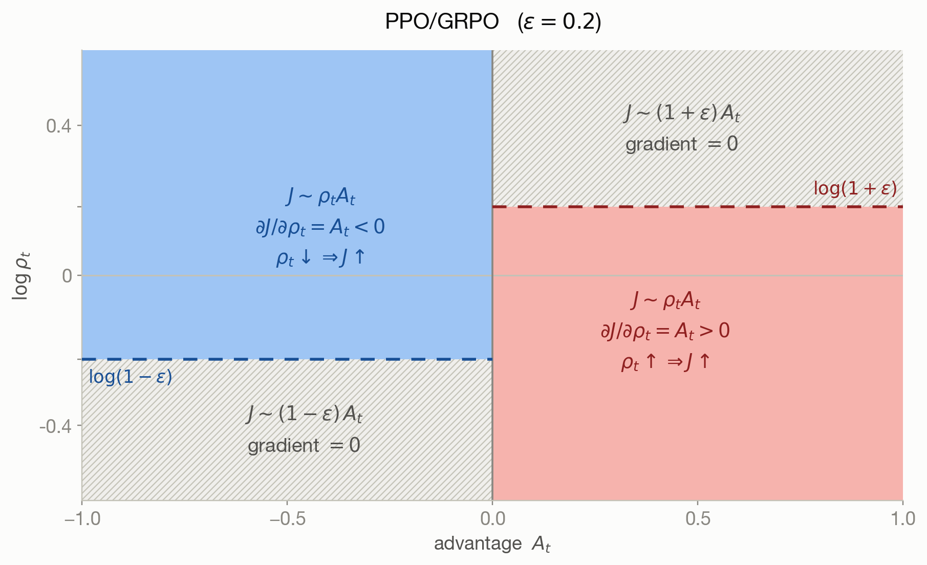
Figure 1 summarizes this behavior. On the $\log\rho_t$ vs. $A_t$ plane, a sampled token falls into one of four regions: in the red region, PPO/GRPO encourages the token by increasing its probability; in the blue region, it discourages the token; in the remaining regions, the gradient on $\rho_t$ is zero, so the token is effectively dropped from the parameter update.

Generalized RL objective

The SAPO paper⁶ gives us a useful way to compare these policy optimization methods. At the token level, write the surrogate objective as

$$J_t(\theta)=f(\rho_t(\theta);A_t)\,A_t. \tag{4}$$

Policy optimization methods, such as PPO/GRPO, DAPO, GSPO, SAO, and SAPO, differ mainly in their choice of the weight function $f$. Taking the gradient of eq. (4),

$$\begin{aligned} \nabla_\theta J_t &= A_t f'(\rho_t;A_t)\,\nabla_\theta\rho_t \\[4pt] &= \underbrace{f'(\rho_t;A_t)}_{\text{method-specific}} \underbrace{ \rho_t\, \overbrace{A_t\nabla_\theta \log\pi_\theta(y_t\mid x,y_{<t})}^{\text{policy gradient}} }_{\text{shared}}. \end{aligned} \tag{5}$$

All methods share the term $\rho_t A_t\nabla_\theta\log\pi_\theta$. They only differ in the gate function $f'(\rho_t;A_t)$ that determines how much learning signal gets through.

Table 1 summarizes the weight function $f$ and gate function $f'$ of some milestone policy optimization methods in LLM RL.

Method	$f(\rho_t;A_t)$	$f'(\rho_t;A_t)$	Insight
PPO (July 2017) / GRPO (February 2024)	$A_t>0:\;\min(\rho_t,1+\epsilon)$ $A_t\leq0:\;\max(\rho_t,1-\epsilon)$	$\mathbf{1}\left[A_t>0,\;\rho_t<1+\epsilon\right]$ $+\;\mathbf{1}\left[A_t<0,\;\rho_t>1-\epsilon\right]$	Hard, asymmetric gating based on the sign of $A_t$
DAPO (March 2025)	$A_t>0:\;\min(\rho_t,1+\epsilon_h)$ $A_t\leq0:\;\max(\rho_t,1-\epsilon_l)$	$\mathbf{1}\left[A_t>0,\;\rho_t<1+\epsilon_h\right]$ $+\;\mathbf{1}\left[A_t<0,\;\rho_t>1-\epsilon_l\right]$	A higher upper bound leaves more room to increase useful low-probability tokens
GSPO (July 2025)	Same as DAPO at $(\rho_s,A_s)$: $A_s>0:\;\min(\rho_s,1+\epsilon_h)$ $A_s\leq0:\;\max(\rho_s,1-\epsilon_l)$	$\mathbf{1}\left[A_s>0,\;\rho_s<1+\epsilon_h\right]$ $+\;\mathbf{1}\left[A_s<0,\;\rho_s>1-\epsilon_l\right]$	One clip decision per response instead of per token
SAPO (November 2025)	$\dfrac{4}{\tau_t}\sigma\left(\tau_t(\rho_t-1)\right)$, $\tau_t=\tau_{\text{pos}}$ if $A_t>0$, else $\tau_{\text{neg}}$	$4\sigma\left(\tau_t(\rho_t-1)\right)\left(1-\sigma\left(\tau_t(\rho_t-1)\right)\right)$ $=\mathrm{sech}^2\left(\tfrac{\tau_t(\rho_t-1)}{2}\right)$	The gate decays smoothly instead of switching abruptly to zero; $\tau_{\text{neg}}>\tau_{\text{pos}}$ makes it decay faster for negative advantages
SAO (July 2026)	$\widetilde f(\rho_t)=\operatorname{clip}(\rho_t,1-\epsilon_l,1+\epsilon_h)$	$\mathbf{1}\left[1-\epsilon_l<\rho_t<1+\epsilon_h\right]$	Both signs are masked whenever the ratio leaves the trust region

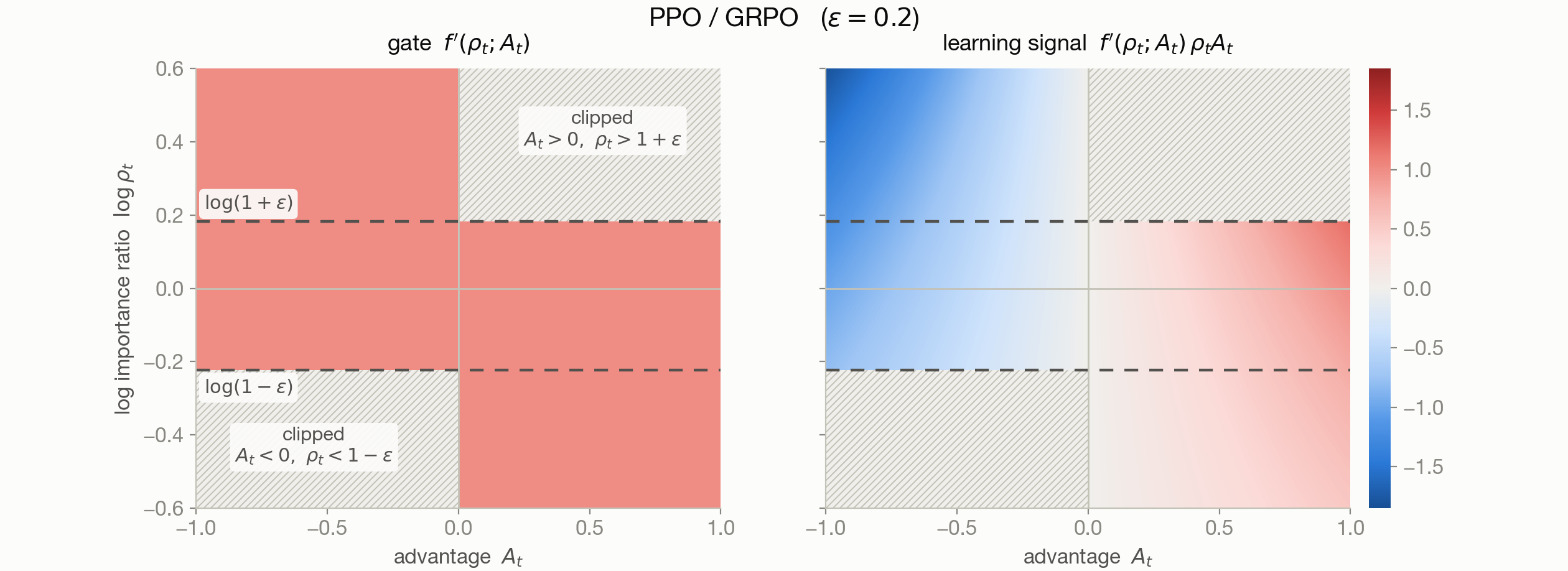
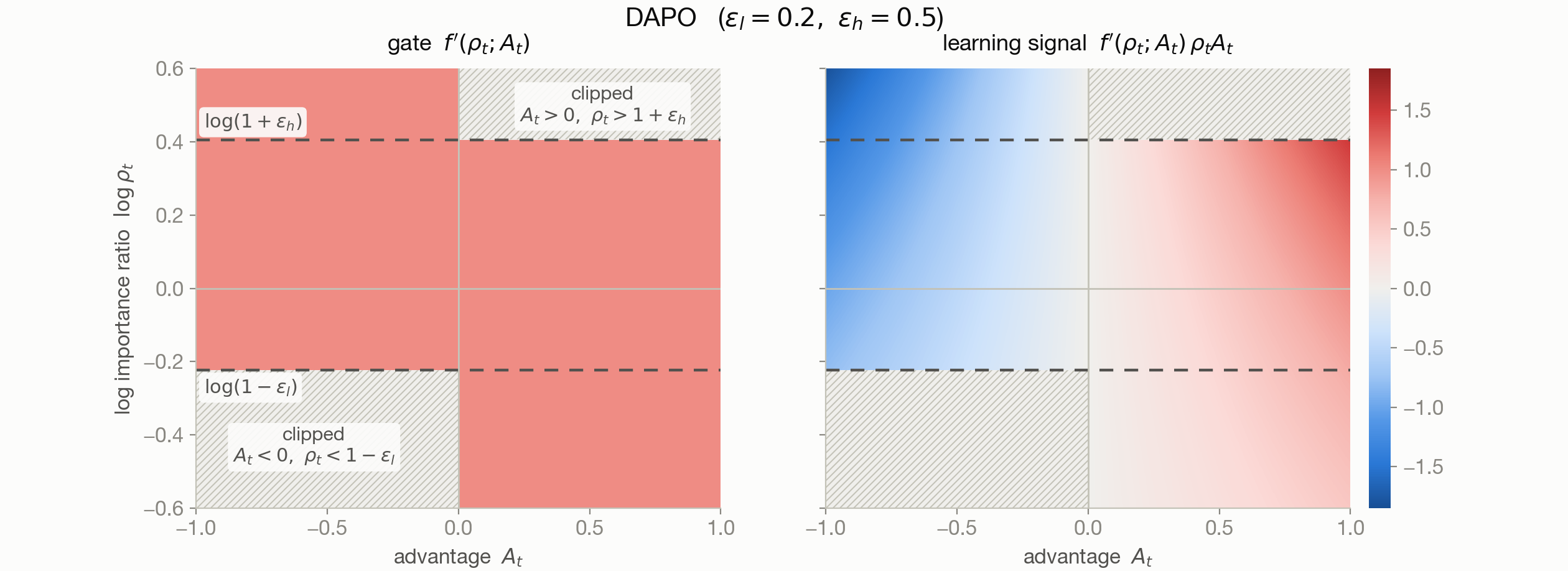
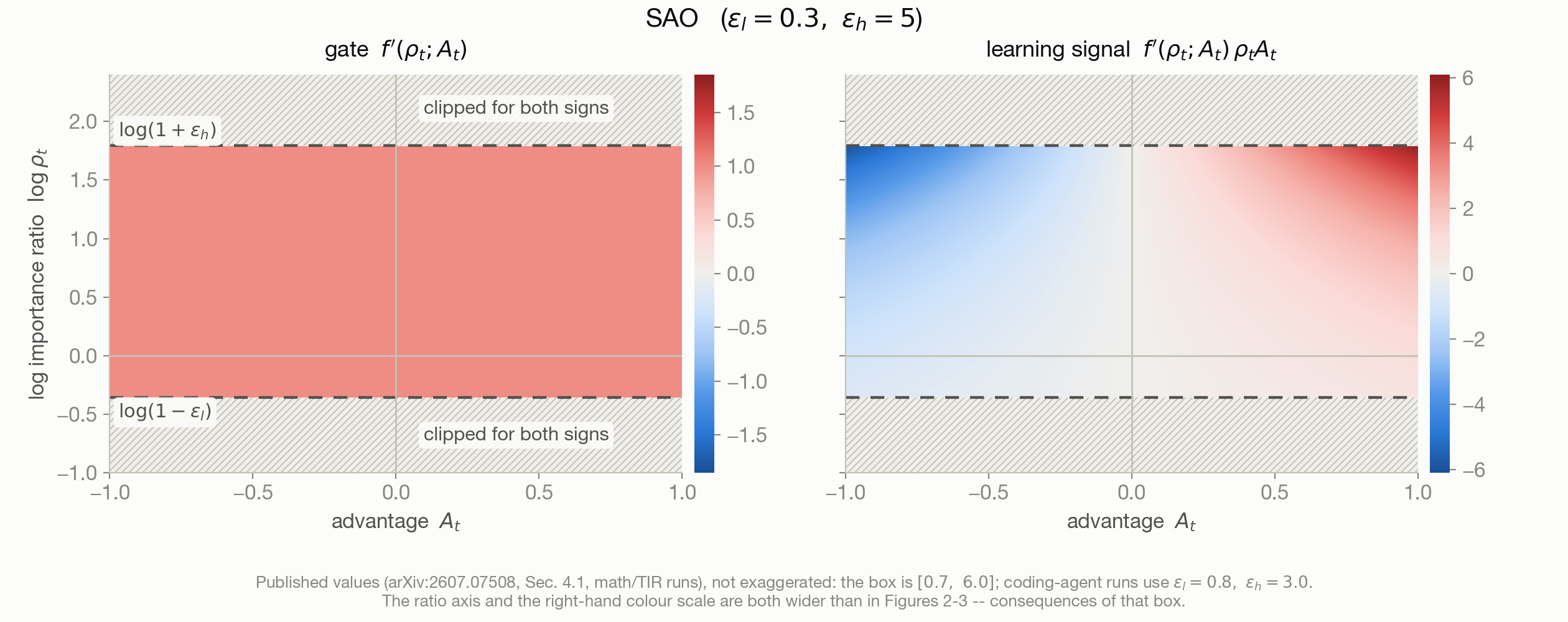
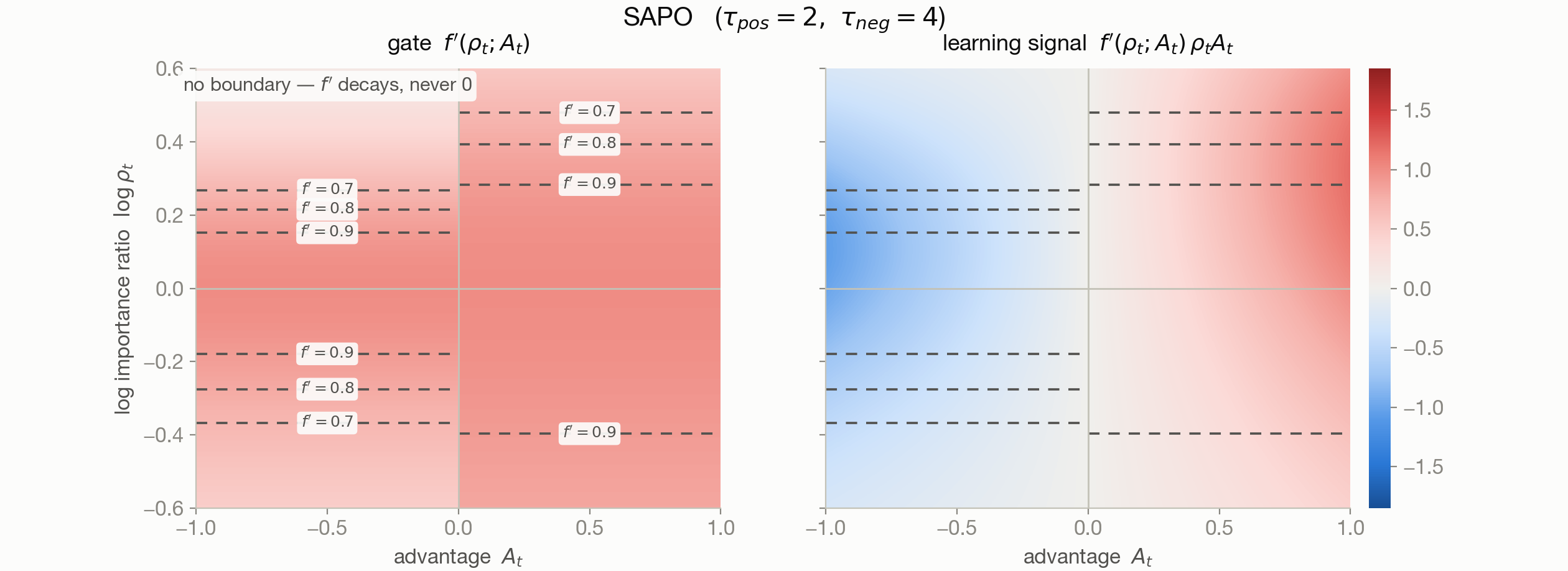
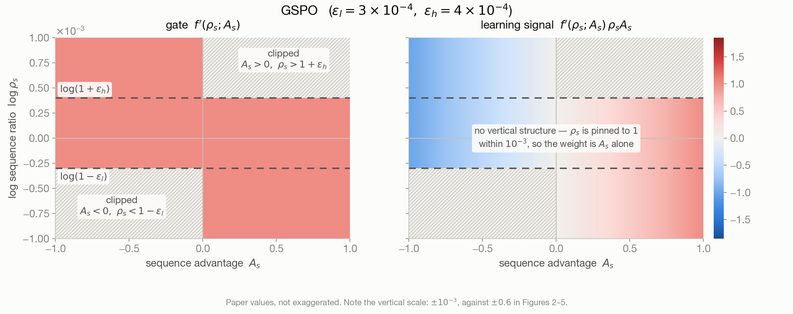
Figures 2–6 plot the gate $f'(\rho_t;A_t)$ and the learning signal $f'(\rho_t;A_t)\,\rho_t A_t$ on the $(A_t,\log\rho_t)$ plane for each method (Figure 6 uses the sequence pair $(A_s,\rho_s)$):

• PPO¹ (Figure 2) clips the importance ratio $\rho_t$: once an update has encouraged a good token or discouraged a bad token enough, the gate drops to zero and the token stops contributing. This keeps policy updates small and training stable.
• GRPO² (Figure 2) adds a group rollout dimension $G$ to the objective. At the token level, its gate is identical to PPO’s.
• DAPO³ (Figure 3) raises the upper clipping threshold $\epsilon_h$, so rare tokens—whose small denominator tends to produce large $\rho_t$ values—are less likely to be clipped prematurely. The extra strip above PPO’s boundary is exactly where the largest learning signals live.
• SAO⁵ (Figure 4) targets asynchronous training, where the current and rollout policies can drift farther apart than in PPO. $\rho_t$ can then deviate substantially from 1, so the gate behaves like a top-hat window, masking both signs whenever the ratio leaves the trust region.
• SAPO⁶ (Figure 5) replaces this hard boundary with a smooth gate. Instead of switching off a token’s contribution once $\rho_t$ crosses a threshold, SAPO lets the weight decay gradually as the ratio moves away from the preferred region.
• GSPO⁴ (Figure 6) is the same move at sequence level: swap $(A_t,\rho_t)$ for sequence level $(A_s,\rho_s)$ with $\rho_s=(\pi_\theta(y\mid x)/\pi_{\mathrm{old}}(y\mid x))^{1/\lvert y\rvert}$—the geometric mean of the token ratios in eq. (1). Note that the shared factor changes as well: $\nabla_\theta\rho_s=\rho_s\cdot\frac{1}{\lvert y\rvert}\sum_t\nabla_\theta\log\pi_\theta(y_t\mid x,y_{<t})$, i.e. every token in the response receives the same length-averaged weight. The gate is DAPO’s asymmetric two-wedge shape, but with GSPO’s clip range ($\epsilon\sim 3\text{–}4\times10^{-4}$) $\rho_s$ stays within $10^{-3}$ of 1, so the learning signal is essentially $A_s$ alone.

Takeaways

Using SAPO’s⁶ generalized form of objective $J$ with weight function $f(\rho_t; A_t)$, learning signals of different RL methods can be shown on the same $(A_t,\log\rho_t)$ plane.

• PPO / GRPO: hard token-level gate.
• DAPO: widens the gate for useful low-probability tokens.
• SAO: keeps only ratios inside a trust region when rollout policies become stale.
• SAPO: turns the hard gate into a smooth one.
• GSPO: moves the same idea from tokens to sequences.

Seen this way, these methods are providing different answers to the same question: which policy-gradient signals should we trust, and how much?